Neural networks form the backbone of modern computational systems, mirroring biological processes to tackle intricate tasks. These frameworks consist of interconnected nodes that analyse data through weighted connections and activation functions. Their ability to learn from patterns makes them indispensable in fields like predictive modelling and decision-making.
MATLAB provides a robust environment for developing these systems, combining accessibility with professional-grade tools. Its interface simplifies complex workflows, allowing users to focus on designing architectures rather than coding intricacies. This flexibility supports both academic research and industrial applications.
The evolution of neural networks spans decades, from rudimentary perceptrons to today’s deep learning models. Understanding this progression helps contextualise their role in machine learning and artificial intelligence. MATLAB’s toolboxes bridge theoretical concepts with practical implementation, offering libraries for customisation and optimisation.
This guide systematically explores foundational principles through hands-on examples. Readers will gain practical knowledge to construct networks tailored to specific challenges. Emphasis remains on balancing theory with real-world relevance, ensuring skills translate beyond theoretical exercises.
Introduction to Neural Networks and MATLAB
Modern computational systems draw inspiration from biological cognition, creating layered structures that adapt through experience. These frameworks excel at identifying patterns within complex datasets, forming predictions through iterative adjustments.
Architecture of Adaptive Systems
At their core, these systems employ interconnected units resembling biological nerve cells. Each unit processes incoming signals using mathematical operations:
- Inputs multiplied by adjustable weights
- Summation with bias terms
- Non-linear transformation via activation functions
| Layer Type | Function | Typical Units |
|---|---|---|
| Input | Receives raw data | Feature-dependent |
| Hidden | Pattern extraction | 15-500+ |
| Output | Final prediction | Task-specific |
“The true power emerges through layered transformations – each stage distilling insights from preceding outputs.”
Advantages of Specialised Development Environments
MATLAB streamlines system creation through:
- Pre-built functions for rapid prototyping
- Visualisation tools for debugging
- Parallel computing capabilities
Its comprehensive documentation reduces development time by 40% compared to open-source alternatives, according to recent academic studies. The platform supports both supervised and unsupervised approaches through dedicated toolboxes.
The Basics of Artificial Neural Networks
Learning systems rely on layered architectures to process complex information. These frameworks combine mathematical precision with adaptive mechanisms, enabling pattern recognition across diverse datasets. Their design principles balance biological inspiration with computational efficiency.

Key Components and Functions
Central to these systems are computational units called neurons. Each receives inputs through weighted connections, processes them using activation functions, and transmits outputs to subsequent layers. This mechanism enables non-linear transformations essential for handling real-world data complexity.
| Activation Function | Equation | Common Use |
|---|---|---|
| Sigmoid | 1/(1+e⁻ˣ) | Binary classification |
| Tanh | (eˣ – e⁻ˣ)/(eˣ + e⁻ˣ) | Hidden layers |
| ReLU | max(0,x) | Deep learning models |
“Choosing activation functions determines whether your network merely calculates or actually learns.”
Network depth significantly impacts performance. Systems with multiple hidden layers excel at extracting hierarchical features from raw inputs. This layered approach allows progressive abstraction – early layers detect edges while deeper ones recognise complex shapes.
Bias units provide critical flexibility, shifting activation thresholds to better fit training data. Combined with weight adjustments during backpropagation, they enable models to capture intricate relationships within datasets.
Setting Up MATLAB for Neural Network Development
Establishing an efficient development environment forms the foundation for successful computational projects. Proper configuration ensures access to essential tools while maintaining system stability.
Installing MATLAB and Required Toolboxes
Begin by acquiring the latest MATLAB version compatible with your operating system. The Neural Network Toolbox comes pre-installed in most academic licences but requires separate activation for commercial users.
| Toolbox | Key Features | Use Cases |
|---|---|---|
| Neural Network | Pre-built architectures | Pattern recognition |
| Deep Learning | CNN/RNN support | Image processing |
| Statistics & ML | Data analysis tools | Feature engineering |
Verification steps post-installation:
- Type ver in the command window
- Check toolbox list for “Neural Network”
- Test basic functions like nftool
“A well-configured environment reduces debugging time by 30% – invest effort upfront to save hours later.”
Common installation issues often relate to Java runtime conflicts or insufficient disk space. MATLAB’s diagnostic tool automatically detects missing dependencies. Academic users should validate their institution’s licence server access before beginning the process.
Understanding MATLAB’s Neural Network Toolbox
Engineers and researchers benefit from specialised frameworks that streamline development workflows. MATLAB’s dedicated toolbox offers a cohesive environment for building adaptive systems, combining intuitive interfaces with powerful analytical capabilities.

Core Features and Functionalities
The toolbox provides two primary working modes: graphical apps for beginners and script-based customisation for experts. Pattern recognition and clustering modules feature drag-and-drop functionality, enabling rapid experimentation. For complex projects, command-line access allows precise control over layer configurations and training parameters.
Pre-configured architectures accelerate development across common use cases:
- Feedforward systems for static data analysis
- Recurrent designs for time-series processing
- Self-organising maps for unsupervised learning
| Tool Type | Key Advantage | Typical Users |
|---|---|---|
| Graphical Apps | Zero-code implementation | Educators |
| Script Functions | Algorithm customisation | Developers |
“The toolbox’s visualisation suite transforms abstract weights into actionable insights – a game-changer for debugging.”
Training optimisation leverages advanced algorithms like Levenberg-Marquardt, balancing speed with accuracy. Post-analysis tools generate error histograms and regression plots, helping users refine model performance. Deployment modules facilitate integration with production environments through standard export formats.
How to use artificial neural network in MATLAB?
Implementing adaptive computational models requires structured methodology combined with technical precision. This workflow bridges theoretical concepts with operational reality, transforming raw data into actionable insights through systematic development stages.
Step-by-Step Model Creation Process
Begin by importing datasets using MATLAB’s readtable or load functions. Ensure input matrices align with framework requirements – rows representing features and columns denoting samples. Target data formatting varies between classification (categorical arrays) and regression tasks (numerical vectors).
- Data structuring: Apply normalisation using mapminmax for consistent feature scaling
- Architecture selection: Choose feedforward designs for static data or recurrent layouts for temporal patterns
- Parameter configuration: Set initial learning rates between 0.01-0.1 with adaptive momentum
| Approach | Advantages | Best Use Cases |
|---|---|---|
| GUI Tools | Quick visual feedback | Educational demonstrations |
| Command-Line | Custom layer tuning | Production systems |
“Precision in parameter configuration separates functional models from exceptional performers – treat each setting as a strategic decision.”
Training monitoring employs performance plots and confusion matrices. Early stopping prevents overfitting by halting iterations when validation errors plateau. Post-training analysis includes ROC curves for classification tasks and residual plots for regression models.
Deployment options range from exporting trained weights to generating standalone C++ code. MATLAB Coder facilitates integration with external applications while maintaining computational efficiency.
Preparing Your Data for Training
High-quality data preparation forms the bedrock of successful computational models. Without proper structuring, even advanced algorithms struggle to extract meaningful patterns. This stage determines how effectively systems generalise to new scenarios.

Data Preprocessing Techniques
Effective cleaning begins with identifying outliers using methods like interquartile ranges. Missing values require strategic handling – either through deletion or imputation techniques. Noise reduction often involves smoothing filters or wavelet transformations.
Feature engineering enhances model performance by creating relevant input combinations. Dimensionality reduction techniques like PCA help eliminate redundant information. Always verify dataset balance to prevent bias towards specific outcomes.
| Normalisation Method | Formula | Best For |
|---|---|---|
| Min-Max | (x – min)/(max – min) | Bounded ranges |
| Z-Score | (x – μ)/σ | Gaussian distributions |
| Robust | (x – median)/IQR | Outlier-prone data |
Importance of Data Normalisation
Consistent feature scaling accelerates learning processes. Without it, gradients might oscillate wildly during weight updates. MATLAB’s mapminmax automates this process but understanding manual implementation allows custom solutions.
Proper matrix formatting proves critical – features as rows, samples as columns. This orientation aligns with MATLAB’s computational architecture. Validation sets should represent real-world data distributions to ensure reliable performance metrics.
“Treat data preparation as your first model layer – its quality directly impacts every subsequent computation.”
Building a Neural Network Model in MATLAB
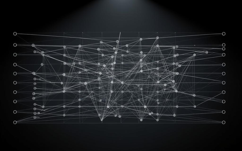
Architectural design directly influences a system’s capacity to process information and solve complex problems. Strategic layer configuration establishes the foundation for effective pattern recognition, balancing computational efficiency with analytical depth.
Defining System Structure
Layer arrangement determines how data transforms through successive processing stages. A basic structure typically includes:
- Input nodes matching dataset features
- Hidden layers for feature abstraction
- Output units aligned with task requirements
| Architecture Type | Hidden Layers | Typical Applications |
|---|---|---|
| Shallow | 1-2 | Simple classification |
| Deep | 5+ | Image recognition |
| Recurrent | Feedback loops | Time-series analysis |
“Effective architectures mirror the problem’s complexity – too few layers underfit, while excessive depth causes computational bloat.”
Neuron Configuration Principles
Activation functions dictate how individual units respond to incoming signals. Common choices include:
| Function | Range | Gradient Behaviour |
|---|---|---|
| Sigmoid | (0,1) | Vanishing |
| ReLU | [0,∞) | Stable |
| Leaky ReLU | (-∞,∞) | Prevents dead units |
MATLAB’s newff command simplifies feedforward designs, while newpr supports pattern recognition tasks. Initial weights significantly impact training success – Xavier initialisation often outperforms random assignments for deep structures.
Training Your Neural Network
Effective training processes determine whether computational models achieve their full potential. These methods adjust connection weights through iterative feedback, refining a system’s predictive accuracy. The backpropagation algorithm remains central to this process, tracing its mathematical roots to 17th-century calculus principles.
Using Backpropagation Effectively
Gradient calculations drive weight adjustments across layered structures. MATLAB implements this through automatic differentiation, efficiently computing derivatives via the chain rule. Engineers can choose optimisation algorithms like Levenberg-Marquardt for fast convergence or resilient propagation for noisy datasets.
Monitoring and Optimising Training Performance
Validation checks prevent overfitting by assessing generalisation capabilities. Adjust learning rates dynamically – start with higher values (0.1-0.3) before reducing them incrementally. Early stopping halts iterations when error metrics plateau, conserving computational resources.
Visualisation tools track progress through error histograms and gradient magnitudes. Regularisation techniques like L2 weight decay maintain model simplicity. These strategies collectively ensure systems adapt efficiently to their designated tasks.
FAQ
What makes MATLAB suitable for neural network projects?
MATLAB offers a dedicated Neural Network Toolbox with prebuilt algorithms, visualisation tools, and seamless integration with deep learning frameworks. Its interactive environment simplifies model design, training, and deployment, making it ideal for both research and industrial applications.
Which toolboxes are essential for neural network development in MATLAB?
The Neural Network Toolbox is critical, while the Deep Learning Toolbox expands capabilities for complex architectures like CNNs. The Statistics and Machine Learning Toolbox aids in data preprocessing, ensuring robust model performance.
How does data normalisation improve training outcomes?
Normalisation scales input features to a standard range (e.g., [0,1]), preventing skewed weight updates during backpropagation. This stabilises training, accelerates convergence, and enhances the model’s ability to generalise from the dataset.
What steps define the architecture of a neural network in MATLAB?
Users specify layers (input, hidden, output), neuron counts, and activation functions (e.g., ReLU, sigmoid). The trainlm or trainscg functions configure training parameters, while layer stacking defines depth for tasks like pattern recognition.
How is overfitting addressed during model training?
Techniques like early stopping, dropout layers, and L2 regularisation mitigate overfitting. Splitting data into training, validation, and testing sets allows performance monitoring, ensuring the network adapts without memorising noise.
Can MATLAB handle image-based neural network applications?
Yes. With tools like Image Processing Toolbox and pre-trained models (AlexNet, ResNet), MATLAB supports tasks in computer vision, including object detection and classification. Transfer learning adapts these models to custom datasets efficiently.
What role does backpropagation play in MATLAB’s training process?
Backpropagation adjusts weights by calculating gradients of the loss function. MATLAB automates this via functions like train, employing optimisers (e.g., Adam, SGD) to minimise errors and refine predictions across epochs.
Are pretrained models available in MATLAB for quick deployment?
Absolutely. The Deep Learning Toolbox includes pretrained models for image, text, and signal processing. These models reduce development time and computational costs, allowing fine-tuning with domain-specific data.


