Modern machine learning thrives on handling patterns that evolve over time. Unlike standard neural networks, which treat each input as isolated, recurrent neural networks (RNNs) specialise in sequences. Think of speech recognition or stock market predictions – scenarios where context matters as much as individual data points.
Traditional models struggle with temporal relationships. RNNs solve this through built-in memory, allowing them to retain information from previous steps. This makes them ideal for analysing streaming data where prior inputs directly shape current outputs.
From voice assistants like Alexa to algorithmic trading systems, RNNs drive innovations requiring dynamic context awareness. Their ability to model dependencies across time steps mirrors human cognition more closely than static approaches. This explains their dominance in fields like natural language processing and weather forecasting.
What sets these architectures apart? The network’s looped design enables continuous learning from sequences. Unlike feedforward models, RNNs process inputs while considering historical context – a game-changer for real-time data interpretation.
Introduction to Sequential Data and Neural Networks
The ability to interpret ordered information separates basic algorithms from advanced predictive models. Sequential data – arranged in meaningful sequences – powers everything from voice assistants to weather forecasts. Unlike isolated data points, these patterns rely on context. Stock prices depend on historical trends, while speech recognition requires understanding syllable order.
Defining Sequential Data
Sequential data appears in nearly every industry. Financial analysts track currency fluctuations over days. Geneticists map DNA base pairs in precise orders. Even Netflix recommendations use viewing histories as sequential inputs. Each element gains meaning from its position and relationship to prior entries.
Time series dominate this category. Daily temperature readings or hourly website traffic showcase how temporal relationships influence analysis. Traditional neural networks struggle here, treating each input as independent rather than interconnected.
Contrasting Feedforward and Recurrent Approaches
Standard neural networks push data in one direction: from input layer to output. This works for static images or single transactions. But sequential tasks demand memory – a system that recalls prior inputs when processing new ones.
RNNs introduce loops, letting information cycle through the network. Imagine reading a sentence word by word while remembering previous context. This cyclical flow enables predictions based on evolving patterns, not just immediate data.
The Fundamentals of Recurrent Neural Networks
Sequential data processing demands architectures that mirror human cognition through temporal patterns. Unlike standard models, recurrent neural networks employ a self-referential loop – their defining feature. This loop acts as a memory lane, letting information from prior steps influence current decisions.

At their core, these systems handle two inputs simultaneously: fresh data and contextual history. Each calculation blends the current input with features from previous inputs. This dual-stream approach enables predictions rooted in evolving context rather than isolated snapshots.
“RNNs transform raw sequences into intelligent forecasts by treating time as a dimension, not an obstacle.”
The magic lies in hidden states – mathematical representations of historical context. These states update at each time step, creating dynamic memory. Weight sharing across steps allows consistent pattern recognition in variable-length sequences, from stock ticks to spoken phrases.
| Feature | Feedforward Networks | Recurrent Networks |
|---|---|---|
| Memory Capacity | None | Contextual history |
| Input Handling | Static snapshots | Time-ordered sequences |
| Parameter Usage | Fixed per layer | Shared across time steps |
Real-world implementations showcase this architecture’s versatility. Language translation tools maintain sentence context through multiple processing stages. Fraud detection systems track transaction patterns across hours or days. The feedback loop turns raw data streams into actionable insights with temporal awareness.
What are recurrent neural networks good for?
From transforming spoken words into text to predicting tomorrow’s stock prices, specialised architectures excel where order matters. These systems decode patterns that unfold across time steps, making them indispensable for tasks requiring temporal awareness.
Speech Recognition Benefits
Voice-activated assistants like Siri demonstrate RNNs’ prowess in processing sequential data. By analysing phoneme sequences – the building blocks of speech – these networks capture contextual relationships between sounds. This allows accurate transcription even with accents or background noise.
Google’s speech-to-text systems use similar principles, converting audio inputs into coherent sentences. The looping mechanism retains context between syllables, mirroring how humans interpret language through cumulative understanding.
Time Series Forecasting Potential
Financial institutions leverage RNNs to predict market trends using historical trading data. By processing thousands of time steps, these models identify subtle patterns invisible to traditional analysis. Weather forecasting systems similarly benefit, combining past atmospheric inputs with current measurements.
Retail giants like Amazon use such architectures for demand planning. Their systems analyse purchase histories and seasonal trends to optimise inventory levels – a task requiring precise interpretation of evolving sequential data.
Advantages of RNNs in Processing Sequential Data
Adaptive architecture gives recurrent systems unmatched flexibility in handling temporal patterns. These models process sequences of any length without structural changes – a critical advantage for real-world applications dealing with unpredictable data streams. Unlike fixed-size architectures, they maintain parameter efficiency through intelligent design choices.
Memory and Parameter Sharing
The secret lies in shared weights across time steps. Each layer reuses identical parameters when processing different inputs, dramatically reducing computational demands. This approach:
- Prevents model bloat with growing sequence lengths
- Enables consistent pattern recognition in variable contexts
- Allows cumulative retention of past information
Financial forecasting systems exemplify this advantage. They analyse years of market data without increasing complexity – the same weights process daily, weekly, and monthly trends.
Integration with Convolutional Neural Networks
Combining temporal and spatial processing unlocks new capabilities. Convolutional layers extract visual features from images, while recurrent components interpret sequential relationships. This hybrid approach powers:
- Video analysis tracking object movements frame-by-frame
- Medical imaging systems correlating scan sequences
- Automated caption generation for visual content
Google’s DeepMind uses such architectures for weather prediction models. Spatial atmospheric patterns merge with temporal progression data, creating forecasts that understand both what’s happening and how it’s changing.
Challenges in Training RNNs
Training RNNs presents unique hurdles that test both computational resources and algorithmic ingenuity. These obstacles stem from their temporal processing nature, creating three primary pain points for developers.
Vanishing Gradient Issue
During training, gradients carrying adjustment signals weaken as they travel backward through time steps. This exponential decay leaves initial layers with negligible updates, effectively freezing early weights. The network consequently struggles to learn long-range dependencies in financial forecasts or multi-sentence text analysis.
Exploding Gradient Problem
The reverse scenario sees gradients ballooning uncontrollably during backpropagation. Unchecked, these runaway values cause drastic weights adjustments that destabilise networks. Sudden spikes in loss functions often indicate this issue, particularly when processing lengthy video sequences.
Computational Complexity Considerations
RNNs process data sequentially, preventing parallelisation advantages seen in convolutional networks. Each time step depends on previous calculations, extending training times exponentially for long sequences like genome patterns.
| Challenge | Primary Cause | Typical Impact |
|---|---|---|
| Vanishing Gradient | Repeated matrix multiplications | Stalled learning in early layers |
| Exploding Gradient | Unstable activation functions | Overshooting optimal weights |
| Compute Demands | Sequential processing | 4x longer training vs CNNs |
Modern solutions like gradient clipping and architectural innovations (LSTM/GRU units) help mitigate these issues. However, practitioners must still balance temporal depth against computational costs when designing sequence models.
Understanding RNN Architectures
Architectural flexibility defines RNNs’ value in temporal data tasks. Four primary configurations govern how these systems process inputs and generate outputs. Each type serves distinct purposes, from classifying static images to translating entire documents.
One-to-One and One-to-Many Configurations
The simplest type neural setup mirrors traditional models. One-to-one architectures handle single input to single output tasks like image classification. No temporal processing occurs – ideal for static data analysis.
One-to-many systems shine in creative applications. These types recurrent neural setups transform individual inputs into sequences. Music generators build entire compositions from initial chords, while image captioning tools convert photos into descriptive paragraphs.
Many-to-One and Many-to-Many Setups
Sentiment analysis exemplifies many-to-one designs. These models digest entire text documents to produce singular outputs like emotion ratings. They aggregate sequential inputs into consolidated judgements.
Machine translation relies on many-to-many configurations. This type neural architecture processes variable-length sequences bidirectionally. Real-time language converters maintain context across sentences, preserving meaning while adjusting structure.
| Configuration | Input Structure | Output Type | Use Cases |
|---|---|---|---|
| One-to-One | Single unit | Single unit | Image classification |
| One-to-Many | Single unit | Sequence | Music generation |
| Many-to-One | Sequence | Single unit | Sentiment analysis |
| Many-to-Many | Sequence | Sequence | Machine translation |
Choosing the right types recurrent neural design depends on data patterns. While one RNN handles isolated decisions, another manages complex interdependencies. Developers match architectures to temporal requirements for optimal performance.
Deep Dive into RNN Variants: LSTM and GRU
Standard RNN architectures face significant challenges when processing lengthy sequence inputs. Advanced variants combat vanishing gradients and memory limitations through intelligent gating systems. Two dominant solutions have emerged in deep learning: streamlined GRUs and sophisticated LSTMs.
Gated Recurrent Units Overview
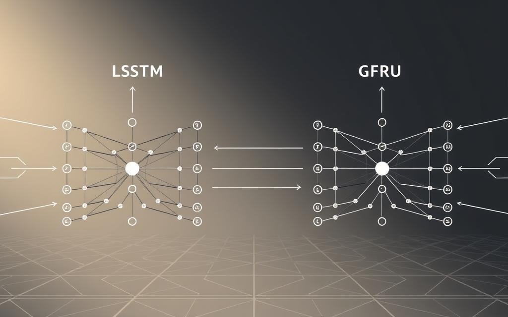
GRUs simplify architecture with just two control mechanisms. The update gate decides how much historical information to retain, balancing past context with fresh inputs. Meanwhile, the reset gate filters outdated details that might distort current analysis.
This dual-gate design achieves:
- Faster training times than traditional architectures
- Efficient handling of medium-range dependencies
- Reduced risk of overfitting in speech recognition tasks
Long Short-Term Memory Mechanism
LSTMs employ three gates for precise memory management. The input gate evaluates new data’s relevance, while the forget gate systematically discards obsolete information. Finally, the output gate determines which insights to feed into subsequent time steps.
| Gate Type | GRU Function | LSTM Role |
|---|---|---|
| Update/Input | Blends old & new data | Filters incoming information |
| Reset/Forget | Removes irrelevant history | Deletes outdated cell content |
| -/Output | N/A | Controls final output delivery |
These mechanisms enable both variants to maintain stable gradients across thousands of processing steps. Financial institutions use LSTMs for decade-spanning market predictions, while GRUs power real-time translation tools needing quick context switches.
Bidirectional RNNs and their Applications
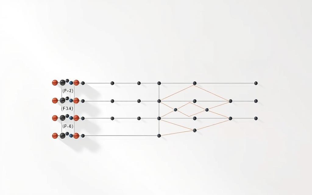
Traditional sequence analysis often overlooks future context. Bidirectional recurrent neural networks (BRNNs) break this limitation by processing data in both temporal directions. This dual perspective proves vital for tasks requiring full sequence awareness.
Processing Past and Future Context
BRNNs deploy two independent neural networks – one analysing input chronologically, the other reverse-engineers the sequence. Their combined outputs create context-rich predictions. Voice assistants use this approach to interpret mumbled words by cross-referencing preceding and following syllables.
Financial models benefit similarly. Analysing stock trends forwards and backwards helps identify hidden patterns. Google’s BERT language model employs bidirectional processing to grasp nuanced word relationships in sentences.
These architectures excel where past information alone proves insufficient. Medical diagnostics systems process patient histories alongside future test projections. Amazon’s Alexa combines both temporal streams to handle interrupted commands mid-sentence.
FAQ
How do recurrent neural networks handle sequential information differently from standard networks?
Unlike feedforward architectures, RNNs use internal memory to process sequences by retaining past information. This allows analysis of temporal patterns in data like speech or stock prices through cyclic connections between layers.
Why are vanishing gradients problematic for training RNNs?
During backpropagation through time, gradients can shrink exponentially, causing earlier time steps to learn slower than later ones. This limits the network’s ability to capture long-range dependencies in sequences like text paragraphs.
What makes LSTMs more effective than basic RNNs for machine translation?
Long short-term memory units employ input, output, and forget gates to regulate information flow. This architecture mitigates vanishing gradients while preserving context over extended sequences – critical for translating multi-sentence content accurately.
Can bidirectional RNNs improve sentiment analysis outcomes?
Yes. By processing data in both forward and backward directions, bidirectional networks capture contextual relationships between words more effectively. This dual perspective enhances accuracy in tasks like emotion classification or named entity recognition.
How do GRUs simplify training compared to traditional RNNs?
Gated recurrent units use reset and update gates instead of separate memory cells, reducing computational complexity. This streamlined design often achieves comparable performance to LSTMs in tasks like speech recognition while using fewer parameters.
Why are RNNs preferred for real-time applications like voice assistants?
Their ability to process streaming data incrementally – rather than requiring full sequences upfront – makes them ideal for low-latency scenarios. This enables immediate responses in dialogue systems or live captioning services.
What techniques address exploding gradients in deep recurrent networks?
Gradient clipping thresholds excessively large updates during optimisation, preventing numerical instability. Architectural solutions like skip connections or layer normalisation also help maintain stable training dynamics.
How do many-to-many configurations benefit video analysis?
These setups process sequential frames as inputs while generating time-stamped outputs, enabling frame-by-frame action recognition. Applications range from sports analytics to autonomous vehicle navigation systems.
